
Blog Post by Yari
March 16th, 2026
There’s no deep altruistic reasoning behind why I do the things I do. I do them simply because I can and after hearing, yet again, about one of my friends dating another person who ended in disappointment, I figured: if machine learning can price risk, it can probably score how much of a red flag the people they are dating are. So get ready, girlie pop. I’m about to make a 30 day behavioral pattern neural network that will help you date better.
There comes a point in every woman’s life where she stares at her phone, half in disbelief, half in delusion, and asks the eternal question: “Is he into me, or just nonchalant?”
*My boyfriend thinks anyone that gives you mixed signals is simply not attracted to your gender. He went into extensive reasoning; he’s AI engineers, so metrics matter to him.*
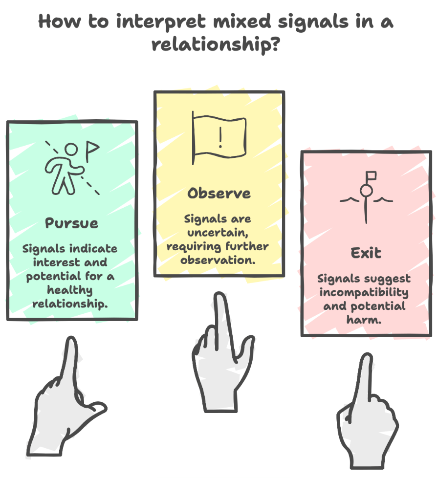
Almost everyone has a situationship, some look like bad friendships; others look like almost relationships that never quite materialize. If only romance came with disclosure statements, quarterly filings, and recommendation ratings from prior users. A fully regularized system looks like the the following:
- Buy (pursue: green flag, pursue)
- Hold (observe: uncertain, observe)
- Sell (exit immediately: red flag, exit)
But it doesn’t. So, I built one.
From an early age, women are taught to interpret mixed signals: a cocktail of affection and avoidance. “He’s mean because he likes you.” “Let’s just go with the flow.” As if you were a passive asset drifting through someone else’s market cycle. I don’t understand the dating obsession with making women suffer simply because they lack candor (honesty). It’s volatile. The emotional equivalent of a candlestick chart, up one day, down the next. Nothing stable enough to model, but just compelling enough to keep you watching.
But we’re better than that. We’re quants. We input data. We measure confidence. We evaluate patterns, not promises and most of all we decode ambiguity.
Once you treat behavior like data, life becomes less chaotic. So, we’ll demystify mixed signals using what they actually are at their core: a behavioral time series using a neural network.
The Asset: Him (I surveyed this)
You meet a guy in NYC. He’s 6’4, finance (just like the song), charming, just self-aware enough to be dangerous. But you think about it for a bit, the reward simply doesn’t outweigh the risk and yet when he invests in you, you feel it, loving the catering you get that lasts max 2 days before suddenly he withdraws. That man right there? High beta. He behaves like the exact type of stock investors warn you about:
- Exciting
- Unpredictable
- Carrying more downside risk than upside potential
When he invests in you, you feel it. Intensity, attention, effort lasts max duration: 48 hours. Then he pulls back. Suddenly, you’re left analyzing a dip you didn’t see coming. The reward feels real. The pattern is not.
The Signal: Micro Behaviors
Volatility isn’t random. The market always leaves traces. Look closer and you’ll see consistent signals:
- Texts at 2 AM that disappear by 2 PM
- Intense compliments that avoid definition
- Plans to a date that cancel with a “sorry, work is crazy.”
- Watching everything you post, initiating nothing. He’s haunting you.
- The he’s “not ready,” but won’t leave you alone.
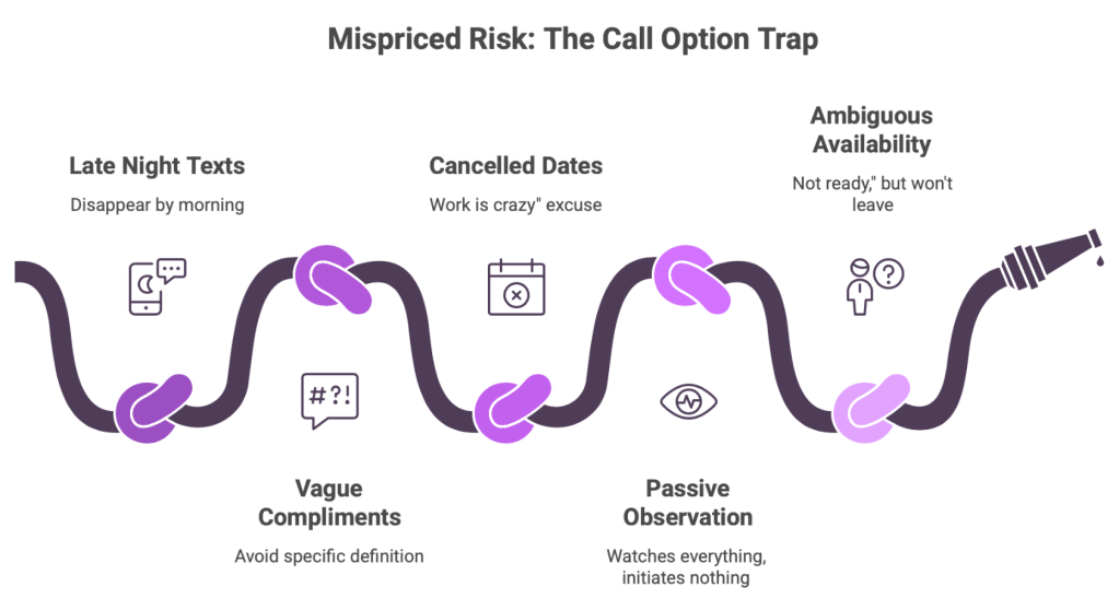
That’s not romance. That’s mispriced risk. Financially speaking, he wants a call option on you without paying the premium. And that’s never a position you want to be in in finance or life.
The Model: Pattern Recognition
Across finance, tech, and AI, one principle holds: Inconsistent signals = unreliable output.
AI models don’t learn from inconsistent labels. Financial models don’t trust incomplete data.
You shouldn’t either. When behavior is inconsistent, don’t analyze the warmth. Analyze the pattern, because mixed signals always converge to one of three outcomes:
- He likes you, but not enough –> Harsh, but liberating.
- He likes you, but he’s emotionally unavailable –> A problem he must solve, not you.
- He likes attention more than accountability –> The most common scenario.
None of these are long positions. Mixed signals are not proof of potential, they are proof of misalignment.
The Trap: Intermittent Reinforcement
So why do people stay? Because mixed signals mimic one of the most addictive systems in behavioral economics: intermittent reward loops.
You get just enough attention to stay hopeful, but never enough stability to feel secure, similar to gambling. Hope makes you creative. Ambiguity makes you analytical. Together, they create delusion disguised as depth. But you don’t need to decode someone who’s aligned. Clarity doesn’t require interpretation.
The Build: A 30 Day Behavioral Model
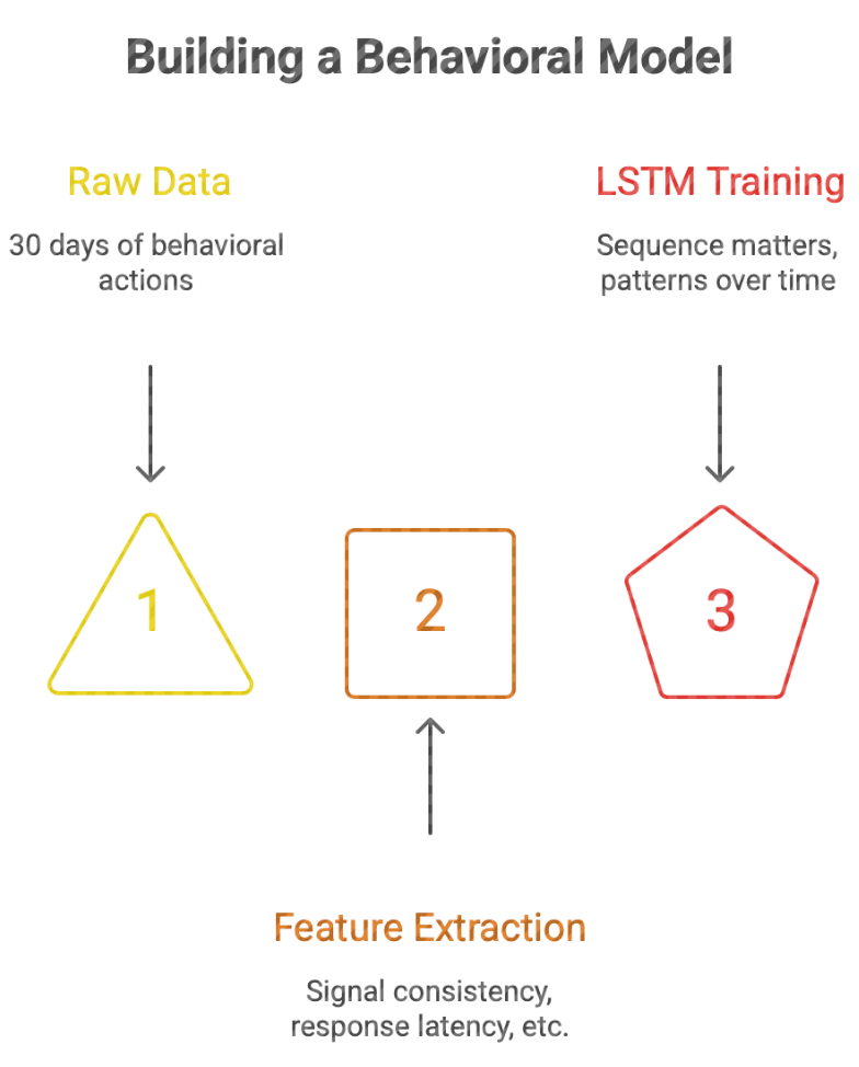
So, let’s formalize it. We take a 30 day window of behavioral data, actions, timing, consistency, and treat it like a financial time series.
Because that’s exactly what it is. We model:
- Signal consistency
- Response latency
- Action to word alignment
- Volatility clustering
And we train an LSTM, not because we’re dramatic, but because sequence matters. This isn’t about one good day or one bad night. It’s about patterns over time.
The Output: Decision Classification
At the end of the model, we ask one question: Is this a Buy, Hold, or Sell?
- Buy (Green Flag): Stable, aligned, consistent behavior
- Hold (Yellow Flag): Unclear, but trending toward stability
- Sell (Red Flag): Volatile, inconsistent, misaligned
And here’s the part no one tells you: If you need a model to justify holding, it’s already a sell.
In finance, assets with persistent volatility, weak fundamentals, and inconsistent signaling are not misunderstood, they’re mispriced risk.
In machine learning, inconsistent input produces unreliable output.
And in life? Mixed signals are not complexity. Don’t chase noise. We don’t price in potential. We don’t hold unstable assets hoping they’ll stabilize. We reallocate. Because the goal was never to predict him. The goal was to protect your portfolio. And any model worth trusting knows one thing: If it doesn’t converge, you don’t keep training it. You discard it.
The Code Breakdown:
Here’s the link to the SELL Dashboard
Here’s the link to the BUY Dashboard
The we define the structure: The month because the market.
n_days = 30 means each history spans one month
n_features = 11 means each day has 11 measurable behaviors
Each case is a 30 day behavioral chart. Mixed signals are a pattern over time. A sequence, a repeated structure of mini letdowns and temporary recoveries. That is exactly why we don’t use one flat row and instead use a time series.
Set feature names:
feature_names = [
    "engagement_volume",
    "latency_hours",
    "execution_ratio",
    "initiative_factor",
    "sentiment_stability",
    "after_hours_activity",
    "default_rate",
    "passive_engagement",
    "disclosure_quality",
    "behavioral_beta",
    "guidance_delivery_spread"
]
These are the factors. Not vibes or excuses.
engagement_volume: His trading volume, how much communication is happening. Is the market alive, or only open at 1:13 AM?
latency_hours: His communication lag, or how long he takes to reply. No one is “so busy” that they can watch your story in real time yet respond 19 hours later.
execution_ratio: the ratio of how many plans are actually honored? This is one of the most important variables, intentions aren’t performances.
initiative_factor: How often he starts the interaction. If all roads lead back to you texting first, that’s not mutual momentum. That’s you acting as both investor and market maker.
sentiment_stability: How emotionally consistent his tone is. If he goes from “you’re special” to spiritual disappearance, the data quality is compromised. We don’t accept ghost signals or false readings.
after_hours_activity: Late night behavior. Some operate like after hours trading. Strange bursts of activity, low governance, bad outcomes. Red Flag.
default_rate: How often he drops the ball, the cancelled plans and missed follow through.
passive_engagement: Lurking social media behavior. A record of every watched stories, liking, the classic low cost access maintenance.
disclosure_quality: How clearly he communicates intent. If every sentence sounds like a legal disclaimer written under emotional distress, this score stays low.
behavioral_beta: His volatility, how unstable is he across time and how much does behavior swing?
guidance_delivery_spread: The gap between what he says and what he does. The spread between projected future performance and actual delivered returns.
Build the spreadsheet of suffering.
X = np.zeros((n_cases, n_days, n_features)) = (1200, 30, 11)
1200 behavioral cases, 30 days each, 11 features per day
The full historical ledger, like the Bloomberg Terminal, but for emotional underperformance.
Simulate Behavioral Types: Buy, Hold, Sell.
Each case gets assigned a hidden profile type: buy, hold, sell. The probabilities are: 30% buy, 30% hold, 40% sell. That means the world this model lives in is already appropriately calibrated.
Create a daily feature generation.
Inside that loop, each day gets generated differently depending on the profile type.
If he’s a buy (Green Flag):
engagement_volume = np.random.normal(10, 2)
latency_hours = np.random.normal(3, 1.5)
execution_ratio = np.random.normal(0.85, 0.08)
This is your consistent. Texts regularly, replies in a sane amount of time. Has follows through, stable emotional tone, decent disclosure quality and low volatility. The same behavior a company with healthy fundamentals and no ongoing federal investigation.
If he’s a hold (Yellow Flag):
engagement_volume = np.random.normal(6, 2.5)
latency_hours = np.random.normal(15, 8)
execution_ratio = np.random.normal(0.50, 0.15)
This is the ambiguity class. Not terrible enough to dump immediately, not strong enough to allocate more capital. Inconsistent, but not always catastrophic. There are moments of effort, confusion, and just enough noise to keep a woman analytical. Dangerous category, actually, hold is where overthinking goes to rent an apartment. Not place to be in, treat this as a SELL(Red Flag).
If he’s a sell (Red Flag return him to the streets)
engagement_volume = np.random.normal(3, 2)
latency_hours = np.random.normal(38, 15)
execution_ratio = np.random.normal(0.20, 0.10)
This is the mixed signal menace. Low engagement, slow replies. High after hours activity, weak execution. The ultimate high behavioral beta. Not a dip but a structurally impaired asset.
Then you’ll have to personalize based on your results it’s how we store the daily values: one day at time.
X[i, d, :] = daily_values
A collection of one day’s behavior case history. By the end, every case has 30 daily observations, that means the model’s not looking at one isolated incident.
It’s looking at the accumulated performance record.
Clipping Values: Keeping the Data in Reality
X[:, :, 0] = np.clip(X[:, :, 0], 0, 25)
X[:, :, 1] = np.clip(X[:, :, 1], 0, 120)
This section prevents impossible values. Because when you simulate with normal distributions, sometimes the math gets a little too creative. You might end up with: negative texts, negative response time, disclosure quality above. And while some do often act outside reasonable bounds, the data still needs guardrails. So, we clip everything into valid ranges, keep the numbers realistic and unlike his explanation for why he “wasn’t ready.”
Label the Full 30 day Sequence: The Final Recommendation
def assign_sequence_label(sequence): month_avg = sequence.mean(axis=0)
Step back and judge the whole month. The code takes the average behavior over the month. Remember one nice day doesn’t reverse 29 days of unstable returns.
Then the code builds a score:
score += month_avg[0] * 0.08
score -= (month_avg[1] / 120.0) * 2.0
score += month_avg[2] * 2.2
This score’s a weighted blend of good and bad behaviors.
Positive contributors, increase the score: engagement volume, execution ratio, initiative, emotional stability, disclosure quality. These are the fundamentals, the reasons to believe the asset may actually be worth holding.
Negative contributors, decrease the score: response latency, after-hours activity, default rate, passive engagement, behavioral beta, guidance delivery spread. These are the warning signs, the quiet little indicators that the chart may be lying to you.
The final classification:
if score >= 2.4:
    return 2
elif score >= 0.8:
    return 1
else:
    return 0
Which maps to:
2 = BUY
1 = HOLD
0 = SELL
He/she gets a rating.
Create the Labels for All Cases
y = np.array([assign_sequence_label(X[i]) for i in range(n_cases)]): This creates the target label for every 30 day case.
So now we have:
X = the month long behavior histories
y = the recommendation class
That’s the entire supervised learning setup. The behavior is the evidence, and the label is the conclusion.
Train Test Split: Because we don’t reward memorization
X_train, X_test, y_train, y_test = train_test_split(
    X, y, test_size=0.25, random_state=42, stratify=y
)
This splits the data into:
75% training
25% testing
The model learns on one set and gets evaluated on another. A model that only memorizes familiar cases is like a friend who gives the same dating advice to every situation. We want the model to generalize, recognize new patterns, and identify fresh nonsense in the wild.
stratify=y keeps the class balance similar in both sets, statistically cleaner.
Standardization: Equalize the Scales
scaler = StandardScaler()
X_train_2d = X_train.reshape(-1, n_features)
X_test_2d = X_test.reshape(-1, n_features)
Different features live on different scales.
For ex:
latency_hours might range from 0 to 120
execution_ratio ranges from 0 to 1
disclosure_quality ranges from 0 to 5
If we feed that directly into a neural net, larger scale variables can dominate unfairly. So, we standardize, but because this is 3D sequence data, we first flatten it into 2D, scale it, and then reshape it back.
X_train_scaled = scaler.fit_transform(X_train_2d).reshape(-1, n_days, n_features)
X_test_scaled = scaler.transform(X_test_2d).reshape(-1, n_days, n_features)
Get on the same numeric playing field and then compare behaviors fairly.
Convert to tensors: use PyTorch
X_train_tensor = torch.tensor(X_train_scaled, dtype=torch.float32)
X_test_tensor = torch.tensor(X_test_scaled, dtype=torch.float32)
y_train_tensor = torch.tensor(y_train, dtype=torch.long)
y_test_tensor = torch.tensor(y_test, dtype=torch.long)
PyTorch doesn’t train on NumPy arrays directly. It needs tensors. That’s the point where the data becomes model ready. Think of it as moving from spreadsheet gossip to institutional grade processing.
Define the LSTM Model: The Nervous System of the Analysis
class MixedSignalsLSTM(nn.Module):
Now we build the neural network, an LSTM, as this is sequence data and the order of days matter. The LSTM remembers prior information across time. Which makes it perfect for mixed signals, because mixed signals are essentially patterned inconsistency.
Inside the model
LSTM Layer
self.lstm = nn.LSTM(
    input_size=input_size,
    hidden_size=hidden_size,
    num_layers=num_layers,
    batch_first=True,
    dropout=dropout
)
This is the memory engine. It reads the 30 days in order and learns which sequences matter.
For ex, it can detect things like: strong start followed by decline, repeated cancellation clusters, after hours spikes after periods of silence, recurring mismatch between, engagement and clarity.
Which is exactly the sort of nonsense women have been manually back testing for years.
Dense Layers
self.fc1 = nn.Linear(hidden_size, 32)
self.relu = nn.ReLU()
self.dropout = nn.Dropout(0.2)
self.fc2 = nn.Linear(32, num_classes)
After the LSTM reads the sequence, the dense layers make the final decision. This is where the model says: “Here’s the rating.”
fc1: compresses the information
ReLU: adds nonlinearity
Dropout: reduces overfitting
fc2: outputs the final class scores
Forward pass
def forward(self, x):
    lstm_out, (hidden, cell) = self.lstm(x)
    x = hidden[-1]
    x = self.fc1(x)
    x = self.relu(x)
    x = self.dropout(x)
    x = self.fc2(x)

    return x
This is how the data moves through the model. The important line is:
x = hidden[-1]
This takes the final hidden state from the last LSTM layer. That summary then gets passed into the dense layers to make the class prediction. Like saying: “I’ve seen enough.”
Loss and Optimizer: How the Model Learns
criterion = nn.CrossEntropyLoss()optimizer = optim.Adam(model.parameters(), lr=0.001)
CrossEntropyLoss
This is the loss function for multi-class classification. It measures how wrong the model is. The worse the predictions, the higher the loss. The lower the loss, the more aligned the model is with the truth.
Adam is the optimizer. It updates the neural network weights to reduce the loss. So, while you once adjusted your standards manually, Adam does it mathematically.
Training Loop: Repeated Exposure Until the Pattern Becomes Clear
epochs = 50

for epoch in range(epochs):
    model.train()
    optimizer.zero_grad()

    outputs = model(X_train_tensor)
    loss = criterion(outputs, y_train_tensor)

    loss.backward()
    optimizer.step()
This is the learning process. Each epoch means the model sees the full training dataset once. Here is what happens each cycle:
model.train(): Puts the network in training mode.
optimizer.zero_grad(): Clears old gradients so they do not pile up.
outputs = model(X_train_tensor): The model makes predictions.
loss = criterion(outputs, y_train_tensor): The model gets judged.
loss.backward(): The errors get sent backward through the network.
optimizer.step(): The weights get updated.
The model keeps reviewing behavior until it learns what instability looks like.
Printing training accuracy
if (epoch + 1) % 5 == 0:
    _, train_pred = torch.max(outputs, 1)
    train_acc = (train_pred == y_train_tensor).float().mean().item()
Every 5 epochs, we check how well the model is doing on training data. It’s like asking: “Has the machine learned enough to identify a menace yet?” Ideally, the answer is yes.
Evaluation: The Real Test
model.eval()

with torch.no_grad():
    test_outputs = model(X_test_tensor)
    _, test_pred = torch.max(test_outputs, 1)
Now we evaluate on unseen data. This is the part that matters, anyone can look smart reviewing familiar chaos but the question is whether the model can identify new cases correctly.
model.eval(): switches off training specific behavior like dropout randomness.
torch.no_grad(): saves memory and tells PyTorch we’re just evaluating, not learning. Then we calculate the metrics.
Accuracy
print(“Accuracy:”, accuracy_score(y_test_np, test_pred_np)): Tells us the overall percentage of correct predictions. A good first glance.
Classification report
print(classification_report(y_test_np, test_pred_np, target_names=["SELL", "HOLD", "BUY"]))
This gives: precision, recall, F1-score for each class.
It tells us not just whether the model is right, but how it is right.
Does it: Over-label people as SELL? Miss too many BUYs? Confuse HOLD and SELL? This tells us whether the machine is balanced or simply bitter.
Confusion matrix
print(confusion_matrix(y_test_np, test_pred_np))
This shows where the model gets confused. Which classes it mixes up and which identifies cleanly. Very useful, because confusion patterns say a lot. Just like in life.
The New Case: One Fresh Month of Behavioral Nonsense
new_case = np.array([[4, 30, 0.30, 0.20, 0.35, 0.70, 0.50, 1, 1.5, 7.5, 0.80],...], dtype=float)
This is one new 30 day case. Thirty rows, one for each day. Eleven features per day. It’s the actual historical record we want the model to judge.
Scaling the New Case: Same Standards for Everyone
new_case_scaled = scaler.transform(new_case)
new_case_scaled = np.expand_dims(new_case_scaled, axis=0)
We scale the new case using the same scaler from training. If we standardize the training data one way and the new data another way, the model gets confused.
np.expand_dims(..., axis=0): adds the batch dimension, so the input becomes: (1, 30, 11)
1 case, 30 days, 11 features. Exactly what the model expects.
Final Prediction: The Rating Arrives
with torch.no_grad():
    pred_logits = model(new_case_tensor)
    pred_probs = torch.softmax(pred_logits, dim=1).numpy()[0]
    pred_class = np.argmax(pred_probs)
This is the final decision pipeline.
pred_logits: Raw class scores from the model.
torch.softmax: Turns them into probabilities.
We don’t just get a class, we get confidence levels. There is a difference between: 51% sell and 97% sell One is a warning, and the other is a full market exit.
Label Mapping: Putting the Verdict in Plain Language
label_map = {
    0: "SELL",
    1: "HOLD",
    2: "BUY "
}
This maps the numeric class back into something readable, while the model may speak in tensors, the girls deserve conclusions.
Print the Output: The Final Investment Memo
print("Recommendation:", label_map[pred_class])
print("Probability Scores:")
print(f"SELL: {pred_probs[0]:.4f}")
print(f"HOLD: {pred_probs[1]:.4f}")
print(f"BUY : {pred_probs[2]:.4f}")
This is the final report. It tells you: the recommendation and the probability of each class
