
Blog post: Yari
Date: July 9th, 2026
Bond analytics sounds like one of those finance phrases designed to make people suddenly remember they have laundry to do. Like something whispered in a Bloomberg Terminal by someone named Chadwick the third, but underneath the jargon, bond analytics is actually pretty relatable.
A bond is basically a financial situationship with a schedule.
You lend money → The bond promises to pay you interest (coupons) and then return the face value at maturity.
Very polite, very structured, very I’ll text you every six months and then pay you back in ten years.
This project prices a fixed coupon bond, solves for yield-to-maturity, builds the cash flow schedule, calculates duration and convexity, visualizes the price yield curve, and compares actual repricing against duration only and duration plus convexity estimates. In simple terms: it answers the bond investor’s favorite question: If interest rates move, how much drama should I expect?
Bond Terms
Bond Model:
- Face value: $1,000
- Coupon rate: 5% annually
- Years to maturity: 10
- Coupon frequency: semiannual
- Market yield: 6%
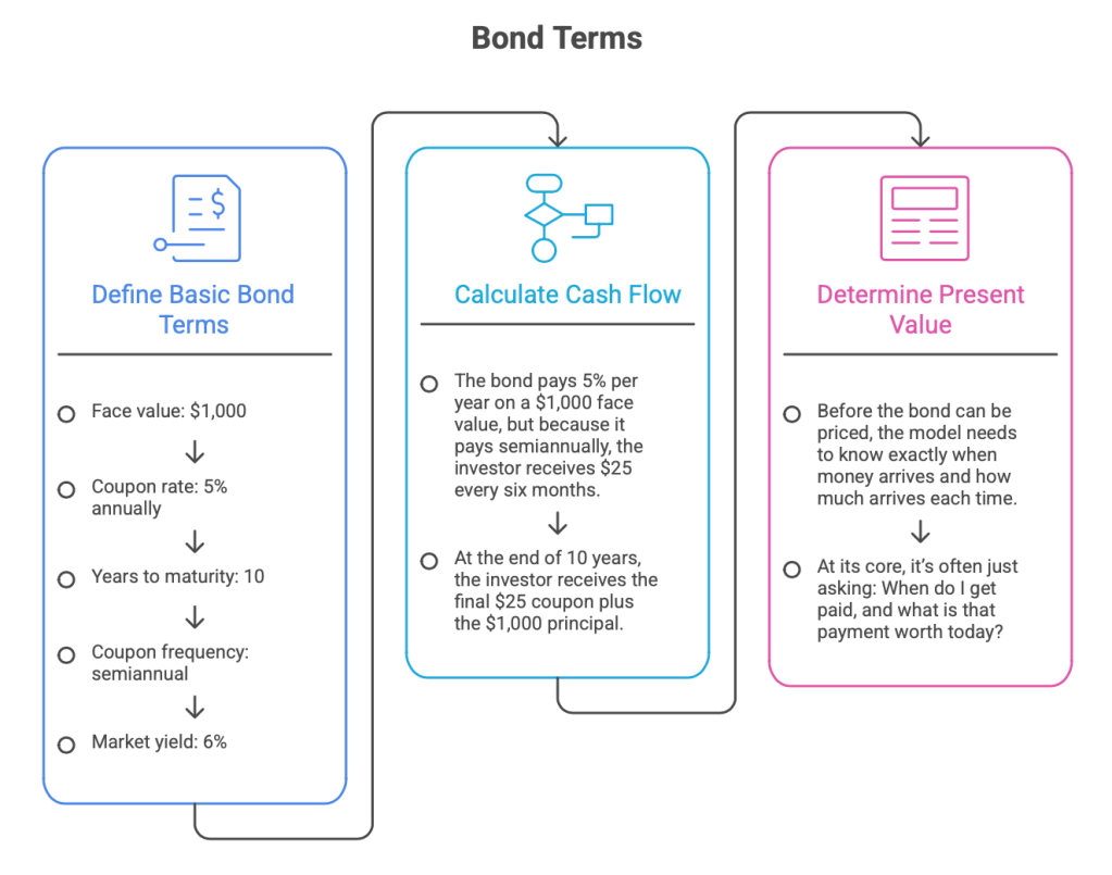
This means the bond pays 5% per year on a $1,000 face value, but because it pays semiannually, the investor receives $25 every six months. At the end of 10 years, the investor receives the final $25 coupon plus the $1,000 principal.
Don’t stress babygirl, the math’s simple, the cash flow backbone of the entire model. Before the bond can be priced, the model needs to know exactly when money arrives and how much arrives each time.
Finance loves to pretend it’s mysterious, but at its core, it’s often just asking: When do I get paid and what’s that payment worth today?
Price From Yield: The Bond’s Reality Check
The first major analytic is price from yield. The idea’s simple: a bond’s price is the present value of all its future cash flows. Every coupon payment and the final principal repayment gets discounted back to today using the market yield.
In the model, the market yield is 6%, while the coupon rate is 5%. That means the market is demanding more return than the bond’s coupon provides. Naturally, the bond has to sell below its $1,000 face value to compensate investors.
The model prices the bond at approximately $925.61. That makes it a discount bond.
This relationship is one of the most important fixed income concepts: when yields rise, bond prices fall. When yields fall, bond prices rise. Bonds and yields are in a long term toxic relationship where one thrives when the other suffers. Very much we need to talk.
Yield-to-Maturity: Reverse Engineering the Market’s Mood
The second major analytic is yield-to-maturity, or YTM. If price-from-yield asks: What is the bond worth if the market yield is 6%?
The YTM then asks the reverse: If the bond is trading at this price, what yield is the market implying?
In the Python code, it’s solved using a Newton Raphson method with a bisection fallback. Conceptually, it’s just the model making educated guesses until the bond price generated by the yield matches the market price. The code says: Try a yield, price the bond, compare it to the target price, adjust the yield. Repeat until the answer is close enough. It’s basically the finance version of trying to guess someone’s coffee order, except the coffee is a 10 year fixed income security and the barista is calculus.
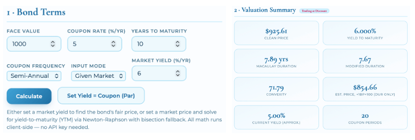
For a market price of $925, the model solves a YTM of about 6.01%. That makes sense because the earlier price at a 6% market yield was around $925.61. The solver is doing exactly what it should: backing into the yield implied by the price. Bonds are often quoted and compared by yield, not just price.
- Price just tells what the bond costs.
- Yield tells what return the market is attaching to that cost.
The Cash Flow Schedule: The Bond’s Calendar Invite
The cash flow schedule is where the bond becomes tangible. The model builds a table with:
- Period, Time in years, Coupon payment, Principal payment,
- Total cash flow, Discount factor and Present value of each cash flow
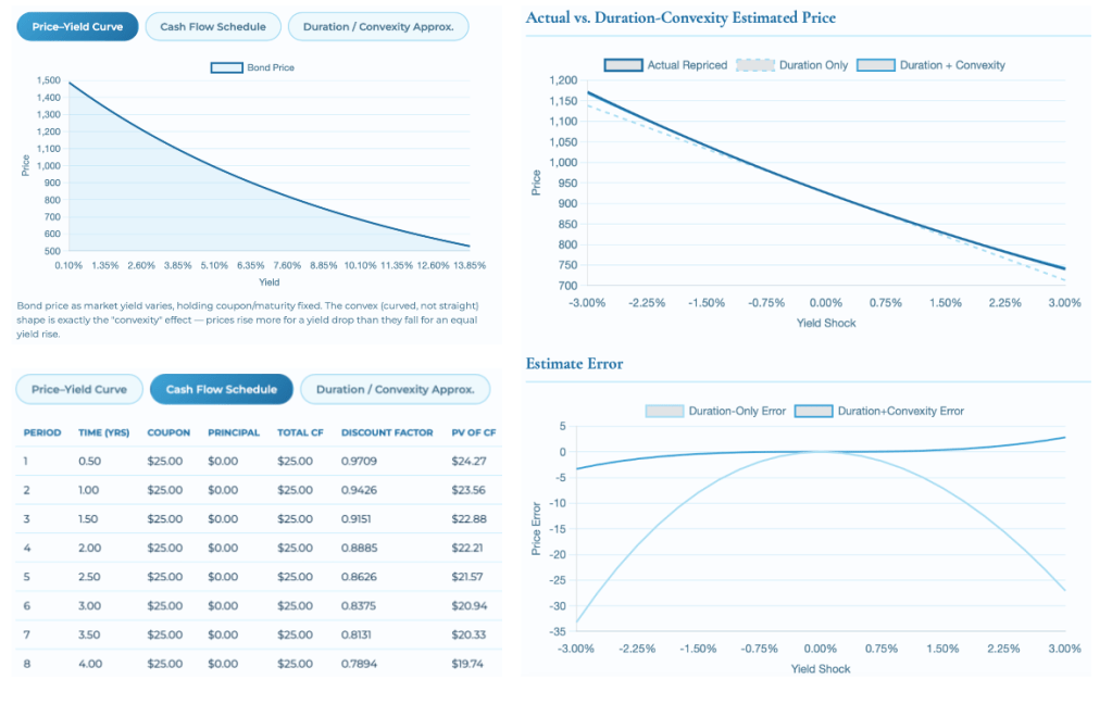
For this bond, each semiannual coupon is $25. The final period includes the last $25 coupon plus the $1,000 principal, making the last cash flow $1,025.
The discount factor tells how much each future payment is worth today. A payment arriving six months from now is worth more today than a payment arriving ten years from now because time, risk, and opportunity cost all exist. Rude, but true. It’s where the model gets useful, it doesn’t just spit out one price, it shows how that price is assembled piece by piece.
The Excel workbook mirrors the same logic, excel is basically the universal language of finance. Python is where the model becomes scalable and elegant while HTML is where it becomes interactive and presentable. But Excel still reigns supreme, it’s where finance crew go hands on verify that the math isn’t mathing. The group chat screenshots of financial modeling, remember all banks are risk adverse, they hate to take risks, so they try their best not to take those risks by bending and curving where they can. Basically: Don’t become a Fintech company, buy a Fintech company and hedge the risk.
Duration: How Sensitive Is This Bond?
Duration’s where bonds get a bit dramatic, while Macaulay duration tells where the weighted average time it takes to receive the bond’s cash flows.
In the model, the Macaulay duration is about 7.89 years. That doesn’t mean the bond matures in 7.89 years. It matures in 10. Duration means that, on a present value weighted basis, the bond behaves like its money is concentrated around 7.89 years. Modified duration then adjusts Macaulay duration to estimate price sensitivity to yield changes. The modified duration is about 7.67.
If yields rise by 1 percentage point, the bond price is expected to fall by roughly 7.67%, using a duration only approximation. If yields fall by 1 percentage point, the bond price is expected to rise by roughly 7.67%.
- A low duration bond is giving: I’m fine.
- A high duration bond is giving: I saw the Fed announcement and need to sit down.
Since this bond has a 10 year maturity and a 5% coupon, it has meaningful interest rate exposure. Not the most dramatic bond in the room, but definitely someone who checks the macro news, and something you need to keep in mind.
DV01: The Price of One Tiny Rate Move
- DV01 = dollar value of one basis point
- A basis point = 0.01%
DV01 estimates how many dollars the bond price changes when yield moves by one basis point.
The formula: Modified Duration × Price × 0.0001
The DV01 is about $0.71.
One basis point move in yield changes the bond’s price by roughly 71 cents. It sounds small, but in institutional portfolios holding millions or billions in face value, DV01 becomes very real, very quick. One basis point is a whisper but in a portfolio turns it into a scream.
Convexity: The Curve Is the Point
Duration is helpful, as it assumes the price yield relationship is linear.
The problem is that bond prices aren’t, they curve.
Convexity is that curve, and it measures how the bond’s duration changes as yields change. In the model, convexity is about 71.79. The exact number’s less important than the idea: convexity improves the estimate because the actual price yield relationship bends. Duration only estimates are decent for small yield changes, but they become less accurate as yield shocks get larger.
A duration only model draws a straight line.
The real bond price moves along a curve. The dashboard compares actual repriced bond values against duration only and duration plus convexity estimates. The result is the fixed income equivalent of realizing the first draft was cute, but the second draft has structure. Duration tells you the first order effect, and Convexity says: Yes, but markets are messier than that, kinda like the two friends in your friendship group that say they never dated out loud but they sure made it awkward that you know they did when one lashed out in the middle of game.
The Price Yield Curve:
The price yield curve is one of the best visuals in the project as it shows the central bond relationship immediately. As yield rises, price falls. But the line isn’t perfectly straight. It curves. That curve is convexity showing up visually. This is why the dashboard is valuable. The concept can sound abstract in a textbook, but once you see the curve yourself, it suddenly clicks.
A yield drop helps the bond more than an equal yield increase hurts it, because of the convex shape. That’s the magic of positive convexity. The bond is basically saying in a tweet: When rates move in my favor, I glowed up harder for my BF to realize I’m hot.
Scenario Analysis:
Scenario analysis takes the model one step further by applying yield shocks from negative to positive changes and comparing three outputs: Actual repriced bond, Duration only estimate, Duration-plus-convexity estimate. This is the risk management part of the project. Instead of only asking what the bond is worth today, it asks what happens if yields move.
It’s important because fixed income isn’t static:
Rates change → Inflation expectations change → Central banks change tone → Markets overreact → Someone on TV says higher for longer and suddenly every bond portfolio starts updating its resume.
The scenario analysis helps show how well the approximations perform. Duration only works reasonably well for small moves, but as shocks get larger, the error grows. Adding convexity reduces the error and tracks the true repriced bond more closely.
In simple terms words, duration is the quick estimate. Convexity is the correction that keeps the estimate from embarrassing itself at dinner.
Market Risk: When the World Starts Acting Expensive
Bonds are calm on paper, but they live in the real world and the real world has a habit of entering the group chat uninvited through things like: Geopolitical tensions, inflation shocks, central bank decisions, recessions, oil price spikes, banking stress, credit downgrades, and investor panic can all affect bond prices.

A bond model can tell you what happens when yields move, but the market decides why yields move and sometimes the reason isn’t elegant:
- War risk, trade tension, sanctions, a surprise inflation print, a central banker choosing violence in a press conference, or investors suddenly deciding they no longer enjoy risk.
It’s less classroom math and more risk radar.
Geopolitical Tensions Rise, investors often move toward safer assets, especially high quality government bonds. That can push yields down and prices up for safer bonds. It’s the classic flight to quality moment: the market gets nervous, and suddenly everyone wants the financial equivalent of a weighted blanket. But not all bonds benefit: Corporate bonds, emerging market bonds, high yield bonds, or bonds tied to unstable regions can get punished. Investors may demand higher yields to compensate for higher perceived risk. When required yields rise, prices fall. That’s the bond market saying: I like income, but I require hazard pay.
Inflation: If it rises, the fixed coupon payments on a bond become less attractive because future dollars lose purchasing power. A $25 coupon sounds cute until groceries, rent, energy, and interest rates all decide to interact. When inflation expectations rise, market yields often rise too, which pushes existing bond prices lower.
Central banks: If the Federal Reserve raises rates or signals that rates may stay higher for longer, existing bonds with lower coupons can lose value because new bonds may offer better yields. That’s why duration matters so much. The higher the duration, the more sensitive the bond is to interest rate changes.
- A short duration bond may react like, ideal but unmanageable.
- A long duration bond reacts like it just read the Fed minutes and needs a chair.
Credit risk: If a company’s financial health weakens, investors may worry that it can’t make coupon payments or repay principal. That can widen credit spreads, meaning investors demand more yield compared with safer bonds. The bond price then falls, not necessarily because general interest rates moved, but because the issuer itself now looks riskier.
Liquidity risk: In stressed markets, some bonds become harder to sell without accepting a lower price. The model may estimate fair value, but the actual market may say, Cute spreadsheet, but can you find a buyer. Liquidity is one of those risks people ignore until they desperately need it.
This is why the scenario analysis in the model is useful. The dashboard doesn’t need to predict every geopolitical event or market shock. Instead, it helps answer a more practical question: If yields move because the world gets messy, how exposed is the bond?
- Duration estimates the first wave of damage or benefit.
- Convexity improves the estimate when the move gets larger.
- DV01 shows the dollar impact of tiny yield changes.
- The price yield curve shows why the relationship is curved, not linear.
The model can’t always stop market drama, but it can help measure how much drama your bond can afford.
The Python Code: The Brain of the Model
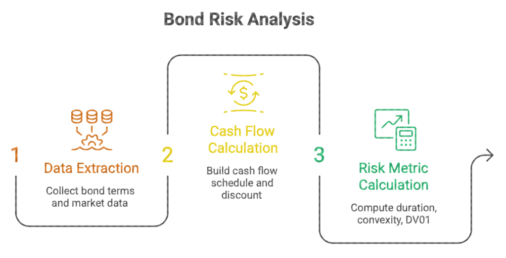
The Jupyter notebook in this article is the analytical engine. NumPy and pandas build cash flows, calculate prices, solve yields, compute duration and convexity, and create charts (you’ll need to familiarize yourself with this when you apply to that quant job).
Main functions:
- build_cash_flows(): Creates the coupon and principal payment schedule.
- price_from_yield(): Discounts every cash flow and sums the present values.
- ytm_from_price(): Solves for the yield that makes the bond’s model price equal to the market price.
- macaulay_duration(): Calculates the weighted average timing of cash flows.
- modified_duration(): Turns Macaulay duration into a yield-sensitivity measure.
- convexity()
Python ETL Pipeline:
In Extraction: the model collects the basic bond terms: Face value, Coupon rate, Years to maturity, Coupon frequency, Market yield or market price. Without them, the model has nothing to price. In the dashboard, these inputs come from the user facing controls. The user enters the face value, coupon rate, maturity, coupon frequency, and then chooses whether they want to price the bond from a given yield or solve for yield from a given price. Conceptually, the extract layer looks like this:
- face_value: 1000
- coupon_rate: 0.05
- years_to_maturity: 10
- coupon_frequency: 2
- market_yield: 0.06
- market_price: 925
The model is only as good as the assumptions it extracts:
- If the coupon frequency is wrong = the cash flows are wrong.
- If the yield is entered incorrectly = the price is wrong.
- If the maturity is off = the duration and convexity are off.
In Transform: the project does the analytical work. The code takes the raw inputs and turns them into structured bond calculations. First, it builds the cash flow schedule. For a semiannual bond, the annual coupon is split into two payments per year. A 5% coupon on a $1,000 bond becomes $50 per year, or $25 every six months. Then the model discounts each future payment back to today using the market yield. That’s where the model calculates:
- Coupon payments, Principal repayment, Total cash flow per period
- Discount factors, Present value of each cash flow, Bond price,
- Yield-to-maturity, Macaulay duration Modified duration, DV01, Convexity,
This is where the project handles two directions of analysis.
First, it calculates price from yield: price = sum(cash_flow / (1 + yield_per_period) x period)
Then it solve yield from price by iterating until the model finds the yield that makes the present value of cash flows equal the market price. The model handles both, sometimes you know the yield and need the price and others the market price and need to infer the yield.
In Load: the model takes the transformed calculations and sends them somewhere useful. In this article, the outputs are loaded into three places: Excel workbook, Python notebook outputs, HTML dashboard (generated for visualization).

